This project is another project from one of my grad school classes. Again, this post is not about any combat robotic activities as I haven't had time in the past semester to do anything combat robotic related. But I thought this project would be interesting to anyone interested in any robotics field.
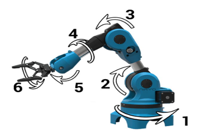
This project centers around a Matlab simulation of a 6 axis robotic manipulator. This robotic arm has 6, rotary joints: 2 at the shoulder, an elbow joint, and 3 rotary joints combined to form a wrist joint of the arm. The arm was modeled in Matlab as a stick figure model of a real arm holding a stylus. The upper and lower arm were 5 units long with a 1 unit length stylus on the end.
This project centers around a Matlab simulation of a 6 axis robotic manipulator. This robotic arm has 6, rotary joints: 2 at the shoulder, an elbow joint, and 3 rotary joints combined to form a wrist joint of the arm. The arm was modeled in Matlab as a stick figure model of a real arm holding a stylus. The upper and lower arm were 5 units long with a 1 unit length stylus on the end.
 | 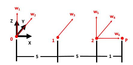 |
The arm was modeled as four points: The base, the elbow, the wrist, and the tip of the stylus. Each of these points was determined using the product of exponentials method that uses the axes of the rotary joints, the angles of each of those axes, and the geometry of the robot when all angles are zero to determine the location and orientation of the end effector of the robot, in this case the stylus. By changing the joint angles and applying the specific product of exponentials formula for this specific manipulator, any point on the robotic arm can be located in 3D space.
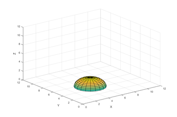
The goal of this simulation was to use this simulated robotic arm to perform obstacle avoidance and path finding in a simulated 3D environment. The base of the arm was to be located at the origin of the 3D environment above. The end of the stylus would start at the point (11, 0, 0) on the right of the screen and algorithmically determine a path to the other side of the space at (0, 11, 0) without colliding with the spherical obstacle in the center of the space or going outside of the space.
The algorithm that this project would be based off is called the probabilistic roadmap algorithm. This algorithm creates a roadmap of connected free configurations of the robot that is used to generate collision free paths in the physical operating space. The process that this algorithm follows begins with the random generation of configurations. In this case, each joint had its own uniform random distribution that the random joint configurations were selected from. The shoulder joints were limited in a way that the elbow of the arm never left the physical space. Using the product of exponentials forward kinematics as described above.
After the random configurations were generated, the configuration had to be evaluated to determine if it was collision free or not. To do this, the location of each of the four main points were calculated. The collision checking algorithm would first check that all of the four points in the arm were within the limits of the physical space above. It would then check that each of the point were in collision with the obstacle in the center of the space. This is a relatively simple process because the obstacle is a sphere with a known location. The process of determining if a point is in collision with the obstacle is as simple as comparing the distance of the point to the center of the sphere with the radius of the obstacle. If the distance between the point and the center is less than the radius of the sphere, the point must be inside of the sphere by definition. If all of the main points of the arm are collision free, the midpoints of the arm segments are evaluated in the same manner. If all of those points pass inspection, the quarter points of the segments are checked. If this configuration passes all of the collision checking tests, the joint angles of the configuration as well as the location of the stylus in the physical space are both recorded and stored.
The whole algorithm of collision checking was a separate algorithm that could be called at multiple points of the process. Because the most difficult part of the physical space to navigate is the area around the obstacle, it would be helpful to generate extra free configurations around the obstacle to make sure there are enough free configurations to easily navigate around the obstacle. This process can be done through a process known as a gaussian sampler. The process starts by first finding a configuration. Based off of the joint angles of this configuration, another configuration is generated. For each joint angle, a gaussian distribution is made that is centered on the previous value. A random value is selected from this distribution that becomes the new joint value. These two configurations are put through the collision checking system. If only one of the two point is found to be collision free, the free configuration and the location of the stylus are stored with the other values. This process generates free points near obstacles as the configuration is only stored when the other configuration is in collision. Because the points must be close to eachother, the free point must be near the obstacle.
 | 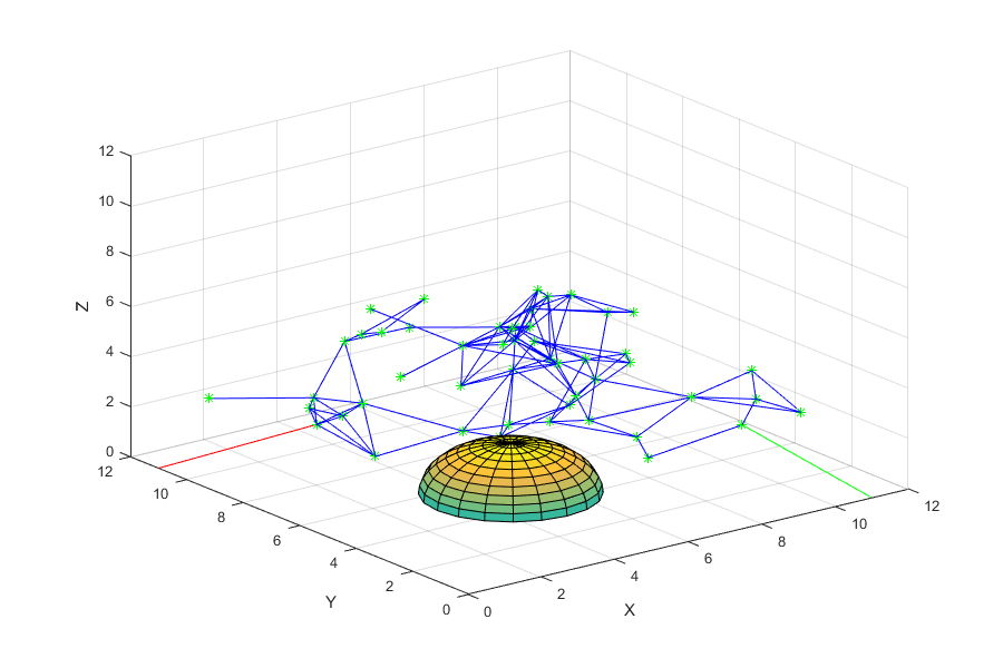 |
Once the requested number of free configurations are found, the next step is connecting the points using a path planner. For every point in the list of free configurations, the distance between the points is calculated. If the points are within a specific distance, a connection is made and the connections are stored in a separate list. This maximum distance for connecting points is a large deciding factor on how dense the roadmap is and how long the algorithm takes. If the distance is too small, the number of free configurations required to create a roadmap capable of completely connecting the physical space increases steeply. This greatly increases the calculation time for the roadmap algorithm. If the distance is too large, the path that is generated is more likely to run into an obstacle and cause the algorithm to fail.
The path planner used in this algorithm is a straight line path planner. The path generated between the points is a straight line in the physical space between the two configurations. Just as the points that are generated must be checked for collisions, so do the paths between them. The paths are checked in a similar manner, starting with the middle point between the two free configuration points. If the distance between the mid point and the center of the obstacle is less than radius of the sphere, than the path would be in collision. If the midpoint passes, the quarter points are also checked. All of these paths and free configuration points are stored and plotted to form a road map.
Once the road map is generated for the space, it can be used to find a path between any two points in the physical space. In this case, only one path is being generated, but many paths could be made from the same roadmap. The first step is to connect the start and goal points with the roadmap. This is as simple as finding the nearest point to the start and goal points in the roadmap. These paths are stored as the beginning and end of the eventual path that the arm takes.
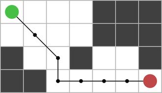
Once the start and goal points are connected, a path between the two points exists, it just needs to be found. This process is done through a custom graphical search algorithm based on the A* search algorithm. The algorithm finds a path when there exists one between a start and goal point. The process begins at a selected node in the roadmap and searches the remaining nodes in the roadmap to find the node that the current node is connected to that is closest to the goal. This process is repeated until the goal point is reached.
This, however is not a foolproof system. This simple system can cause the path to get stuck in dead end path where the only way to reach the goal is to retrace the path back to another path that can reach the goal. The algorithm will always start by following the path that follows the connected node that is closest to the goal, keeping track of the nodes in the path. If there are no connected nodes that have not already been traveled to on that path, that node is labeled as a dead end node. The search process than restarts avoiding the dead end nodes until the goal or another dead end node is reached. This repetitive cycle of trying to find the shortest path while avoiding dead end nodes will eventually find a path if there exists one.
This, however is not a foolproof system. This simple system can cause the path to get stuck in dead end path where the only way to reach the goal is to retrace the path back to another path that can reach the goal. The algorithm will always start by following the path that follows the connected node that is closest to the goal, keeping track of the nodes in the path. If there are no connected nodes that have not already been traveled to on that path, that node is labeled as a dead end node. The search process than restarts avoiding the dead end nodes until the goal or another dead end node is reached. This repetitive cycle of trying to find the shortest path while avoiding dead end nodes will eventually find a path if there exists one.
| | |
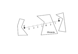
At this point, the path has been generated. The final step is visualization. The Matlab program graphs the roadmap and the the arm and the final path as it traverses along to the goal orientation. The video results can be seen above.
This project was relatively simple as it had a 1 month timeline, but could be improved for more powerful path finding in the same system. By using a more detailed path planner and edge finder that are based on the joint angles instead of the physical distance of the nodes and a straight line between them, the simulation can more realistically model the motions of a physical robotic arm. As you can see a lot of the free configurations tend to be in the middle of the space as it is more probable to find free configurations in this space based on the joint distributions. This could be adjusted by making non uniform distributions or using a resampling process based off of the location of the points or some other method to change the distribution of the nodes.
This project was relatively simple as it had a 1 month timeline, but could be improved for more powerful path finding in the same system. By using a more detailed path planner and edge finder that are based on the joint angles instead of the physical distance of the nodes and a straight line between them, the simulation can more realistically model the motions of a physical robotic arm. As you can see a lot of the free configurations tend to be in the middle of the space as it is more probable to find free configurations in this space based on the joint distributions. This could be adjusted by making non uniform distributions or using a resampling process based off of the location of the points or some other method to change the distribution of the nodes.
 RSS Feed
